语义分割与数据集
Semantic Segmentation and the Dataset
在目标检测问题中,我们只使用矩形边界框来标记和预测图像中的对象。在这一节中,我们将对不同的语义区域进行语义分割。这些语义区域在像素级标记和预测对象。图1显示了一个语义分割的图像,区域标记为“dog”、“cat”和“background”。如您所见,与目标检测相比,语义分割使用像素级边界标记区域,以获得更高的精度。
Fig. 1. Semantically-segmented image, with areas labeled “dog”, “cat”, and “background”.
Image Segmentation and Instance Segmentation
在计算机视觉领域,语义分割有两种重要的方法:图像分割和实例分割。这里,我们将把这些概念与语义分割区分开来,具体如下:
图像分割将一幅图像分成几个组成区域。这种方法通常利用图像中像素之间的相关性。在训练期间,图像像素不需要标签。然而,在预测过程中,这种方法不能保证分割区域具有我们想要的语义。如果输入图像,图像分割可能会将狗分成两个区域,一个覆盖狗的嘴和眼睛,黑色是突出的颜色,另一个覆盖狗的其余部分,黄色是突出的颜色。
实例分割也称为同步检测与分割。该方法尝试识别图像中每个对象实例的像素级区域。与语义分割不同,实例分割不仅区分语义,而且区分不同的对象实例。如果一幅图像包含两条狗,实例分割将区分哪些像素属于哪只狗。
The Pascal VOC Semantic Segmentation Dataset
在语义分割领域,一个重要的数据集是Pascal VOC。为了更好地理解这个数据集,我们必须首先导入实验所需的包或模块。
%matplotlib inline
from d2l
import mxnet as d2l
from mxnet
import gluon, image, np, npx
import os
npx.set_np()
原始站点可能不稳定,因此我们从镜像站点下载数据。该存档文件约为2GB,因此需要一些时间来下载。解压缩归档文件后,数据集位于…/data/VOCdevkit/VOC路径中。
#@save
d2l.DATA_HUB[‘voc’] = (d2l.DATA_URL + ‘VOCtrainval_11-May-.tar’,
‘4e443f8a2eca6b1dac8a6c57641b67dd40621a49’)
voc_dir = d2l.download_extract(‘voc’, ‘VOCdevkit/VOC’)
转到…/data/VOCdevkit/VOC查看数据集的不同部分。ImageSets/Segmentation路径包含指定训练和测试示例的文本文件。JPEGImages和SegmentationClass路径分别包含示例输入图像和标签。这些标签也是图像格式的,与它们对应的输入图像具有相同的尺寸。在标签中,颜色相同的像素属于同一语义范畴。下面定义的read_voc_images函数将所有输入图像和标签读入内存。
#@save
def read_voc_images(voc_dir, is_train=True):
"""Read all VOC feature and label images."""txt_fname = os.path.join(voc_dir, 'ImageSets', 'Segmentation','train.txt' if is_train else 'val.txt')with open(txt_fname, 'r') as f:images = f.read().split()features, labels = [], []for i, fname in enumerate(images):features.append(image.imread(os.path.join(voc_dir, 'JPEGImages', '%s.jpg' % fname)))labels.append(image.imread(os.path.join(voc_dir, 'SegmentationClass', '%s.png' % fname)))return features, labels
train_features, train_labels = read_voc_images(voc_dir, True)
我们绘制前五个输入图像及其标签。在标签图像中,白色代表边界,黑色代表背景。其他颜色对应不同的类别。
n = 5
imgs = train_features[0:n] + train_labels[0:n]
d2l.show_images(imgs, 2, n);
接下来,我们将列出标签中的每个RGB颜色值及其标记的类别。
#@save
VOC_COLORMAP = [[0, 0, 0], [128, 0, 0], [0, 128, 0], [128, 128, 0],
[0, 0, 128], [128, 0, 128], [0, 128, 128], [128, 128, 128],[64, 0, 0], [192, 0, 0], [64, 128, 0], [192, 128, 0],[64, 0, 128], [192, 0, 128], [64, 128, 128], [192, 128, 128],[0, 64, 0], [128, 64, 0], [0, 192, 0], [128, 192, 0],[0, 64, 128]]
#@save
VOC_CLASSES = [‘background’, ‘aeroplane’, ‘bicycle’, ‘bird’, ‘boat’,
'bottle', 'bus', 'car', 'cat', 'chair', 'cow','diningtable', 'dog', 'horse', 'motorbike', 'person','potted plant', 'sheep', 'sofa', 'train', 'tv/monitor']
在定义了上面的两个常量之后,我们可以很容易地找到标签中每个像素的类别索引。
#@save
def build_colormap2label():
"""Build an RGB color to label mapping for
segmentation."""
colormap2label = np.zeros(256 ** 3)for i, colormap in enumerate(VOC_COLORMAP):colormap2label[(colormap[0]*256 + colormap[1])*256 + colormap[2]] = ireturn colormap2label
#@save
def voc_label_indices(colormap, colormap2label):
"""Map an RGB color to a label."""colormap = colormap.astype(np.int32)idx = ((colormap[:, :, 0] * 256 + colormap[:, :, 1]) * 256+ colormap[:, :, 2])
return colormap2label[idx]
例如,在第一个示例图像中,飞机前部的类别索引为1,背景的索引为0。
y = voc_label_indices(train_labels[0], build_colormap2label())
y[105:115, 130:140], VOC_CLASSES[1]
(array([[0., 0., 0., 0., 0., 0., 0., 0., 0., 1.],
[0., 0., 0., 0., 0., 0., 0., 1., 1., 1.],[0., 0., 0., 0., 0., 0., 1., 1., 1., 1.],[0., 0., 0., 0., 0., 1., 1., 1., 1., 1.],[0., 0., 0., 0., 0., 1., 1., 1., 1., 1.],[0., 0., 0., 0., 1., 1., 1., 1., 1., 1.],[0., 0., 0., 0., 0., 1., 1., 1., 1., 1.],[0., 0., 0., 0., 0., 1., 1., 1., 1., 1.],[0., 0., 0., 0., 0., 0., 1., 1., 1., 1.],[0., 0., 0., 0., 0., 0., 0., 0., 1., 1.]]),
‘aeroplane’)
2.1. Data Preprocessing
在前面的章节中,我们缩放图像以使它们适合模型的输入形状。在语义分割中,这种方法需要将预测的像素类别重新映射回原始大小的输入图像。要精确地做到这一点是非常困难的,尤其是在具有不同语义的分段区域中。为了避免这个问题,我们裁剪图像以设置尺寸,而不缩放它们。具体来说,我们使用图像增强中使用的随机裁剪方法从输入图像及其标签中裁剪出相同的区域。
#@save
def voc_rand_crop(feature, label, height, width):
"""Randomly crop for both feature and label
images."""
feature, rect = image.random_crop(feature, (width, height))label = image.fixed_crop(label, *rect)return feature, label
imgs = []
for _ in range(n):
imgs += voc_rand_crop(train_features[0], train_labels[0], 200, 300)
d2l.show_images(imgs[::2] + imgs[1::2], 2, n);
2.2. Dataset Classes for Custom Semantic Segmentation
我们使用gloon提供的继承数据集类来定制语义分段数据集类VOCSegDataset。通过实现thegetitemfunction函数,我们可以从数据集中任意访问索引idx和每个像素的类别索引的输入图像。由于数据集中的某些图像可能小于为随机裁剪指定的输出尺寸,因此必须使用自定义筛选函数删除这些示例。此外,我们定义了normalize_image函数来规范输入图像的三个RGB通道中的每一个。
#@save
class VOCSegDataset(gluon.data.Dataset):
"""A customized dataset to load VOC
dataset."""
def __init__(self, is_train, crop_size, voc_dir):self.rgb_mean = np.array([0.485, 0.456, 0.406])self.rgb_std = np.array([0.229, 0.224, 0.225])self.crop_size = crop_sizefeatures, labels = read_voc_images(voc_dir, is_train=is_train)self.features = [self.normalize_image(feature)for feature in self.filter(features)]self.labels = self.filter(labels)self.colormap2label = build_colormap2label()print('read ' + str(len(self.features)) + ' examples')def normalize_image(self, img):return (img.astype('float32') / 255 - self.rgb_mean) / self.rgb_stddef filter(self, imgs):return [img for img in imgs if (img.shape[0] >= self.crop_size[0] andimg.shape[1] >= self.crop_size[1])]def __getitem__(self, idx):feature, label = voc_rand_crop(self.features[idx], self.labels[idx],*self.crop_size)return (feature.transpose(2, 0, 1),voc_label_indices(label, self.colormap2label))def __len__(self):return len(self.features)
2.3. Reading the Dataset
使用定制的VOCSegDataset类,我们创建训练集和测试集实例。我们假设随机裁剪操作会输出形状中的图像
320×480个
320×480个 .
下面,我们可以看到训练和测试集中保留的示例数。
crop_size = (320, 480)
voc_train = VOCSegDataset(True, crop_size, voc_dir)
voc_test = VOCSegDataset(False, crop_size, voc_dir)
read 1114 examples
read 1078 examples
我们将批处理大小设置为64,并为训练集和测试集定义迭代器。打印第一个小批量的形状。与图像分类和对象识别不同,这里的标签是三维数组。
batch_size = 64
train_iter = gluon.data.DataLoader(voc_train, batch_size, shuffle=True,
last_batch='discard',num_workers=d2l.get_dataloader_workers())
for X, Y in train_iter:
print(X.shape)print(Y.shape)break
(64, 3, 320, 480)
(64, 320, 480)
2.4. Putting
All Things Together
最后,我们下载并定义数据集加载程序。
#@save
def load_data_voc(batch_size, crop_size):
"""Download and load the VOC semantic
dataset."""
voc_dir = d2l.download_extract('voc', os.path.join('VOCdevkit', 'VOC'))num_workers = d2l.get_dataloader_workers()train_iter = gluon.data.DataLoader(VOCSegDataset(True, crop_size, voc_dir), batch_size,shuffle=True, last_batch='discard', num_workers=num_workers)test_iter = gluon.data.DataLoader(VOCSegDataset(False, crop_size, voc_dir), batch_size,last_batch='discard', num_workers=num_workers)return train_iter, test_iter
Summary
语义分割研究如何将图像分割成具有不同语义类别的区域。
在语义分割领域,一个重要的数据集是Pascal VOC。
由于语义分割中的输入图像和标签在像素级有一对一的对应关系,所以我们将它们随机裁剪成固定的大小,而不是缩放它们。